Release candidate for LabPlot 2.1.0
With the upcomming release we decided to change the numbering schema. Starting from now, every time we implement new features, we increase the second digit in the version string. The third digit will be reserved for patch (hot fix) releases without any new features. The major number will be increased on any worldshaking events like new architecture for Qt/KDE, etc. This time, besides many bug fixing and performance improvements, we implemented many new features. – so, it’s going to be 2.1.0.
Today we want to announce the release candidate for v2.1.0. We’ll spend the next couple of days with testing and polishment. No additional features will be implemented during this time. If no bigger issues will be found, we’ll release v2.1.0 soon. The source code of the release candidate is available here. Everybody is welcome to test and to provide any kind of feedback on the new functionality we’re going to describe shortly in the following.
Matrix:
For handling of matrix-like data we introduced a new data container. This matrix data container is presented like a table or, alternatively, as a two-dimensional greyscale image. The elements of such a table/matrix can be thought as being the Z-values, Z=Z(X,Y), with X and Y values being the row and column numbers, respectively. The transition from the row and column numbers to the logical coordinates is done via an explicit user-defined mapping of both worlds.
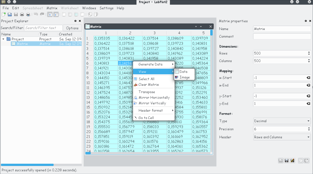
The most prominent application of such a data container one can think of is plotting of 3D-data. So, this new functionality can be regarded as one of the preparation steps towards 3D-plotting in LabPlot. More on this in Minh’s recent blog.
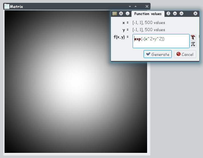
The matrix data can either be entered manually or via an import from an external file. Similar to the data generation for a column in a spreadsheet, the matrix can be filled with constant values or via a formula, too. The screenshot below shows the image view of a matrix together with the formula that was used to generate the matrix elements:
Spreadsheet:
The handling and generation of data in the spreadsheet also got some attention. New operations on columns in the spreadsheet were implemented – reverse, drop and mask values. When specifying which values to drop or to mask, several operators (“equal to”, “greater then”, “lesser then”, etc.) are available. These operations can help to remove (or to hide) some outliers in the data set prior to, e.g., performing a fit to this data set.
Furthermore, the generation of new data via a mathematical expression in spreadsheet was extended to support multiple variables. Now it is possible to define a multivariant function and to provide a data set (a column in a spreadsheet) for each of the variables. The corresponding dialog supports the creation of arbitrary number of variables.
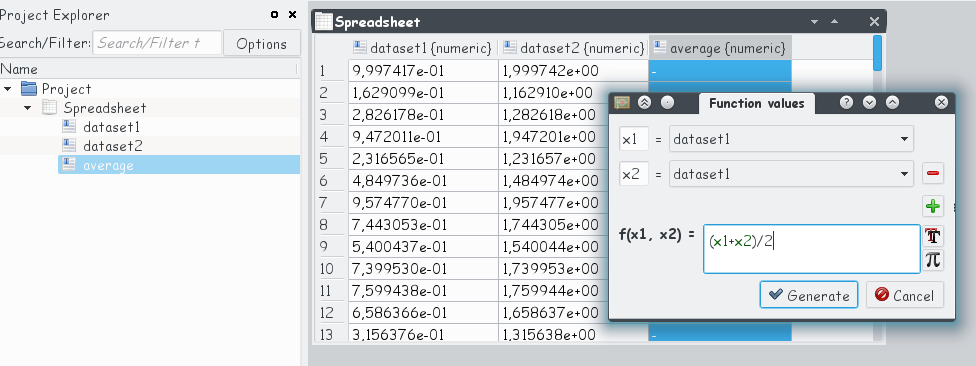
Formula used to generate the values in the column, the names of the variables and the provided columns for each of the parameters are saved and can be changed in the formula dialog afterwords again, if required.
Workbook:
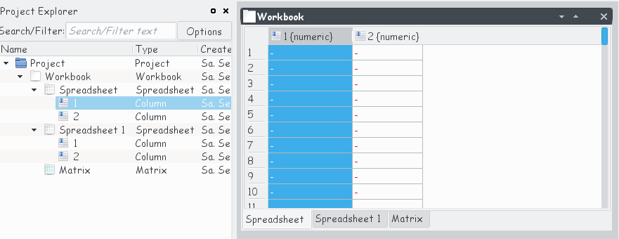
To help the user to better organize and to group different data containers (Spreadsheet and Matrix) we introduced a new object Workbook. This object serves as the parent container for multiple Spreadsheet– and/or Matrix-objects and puts them together in a view with multiple tabs. With folders it is already possible to bring some structure in the project explorer and to, e.g., group together several somehow interconnected spreadsheets with data stemming from text files of similar origin like red, green and blue values of an image imported into three different matrices, etc. With Workbook the user gets now the possibility for another additional grouping.
Data Import:
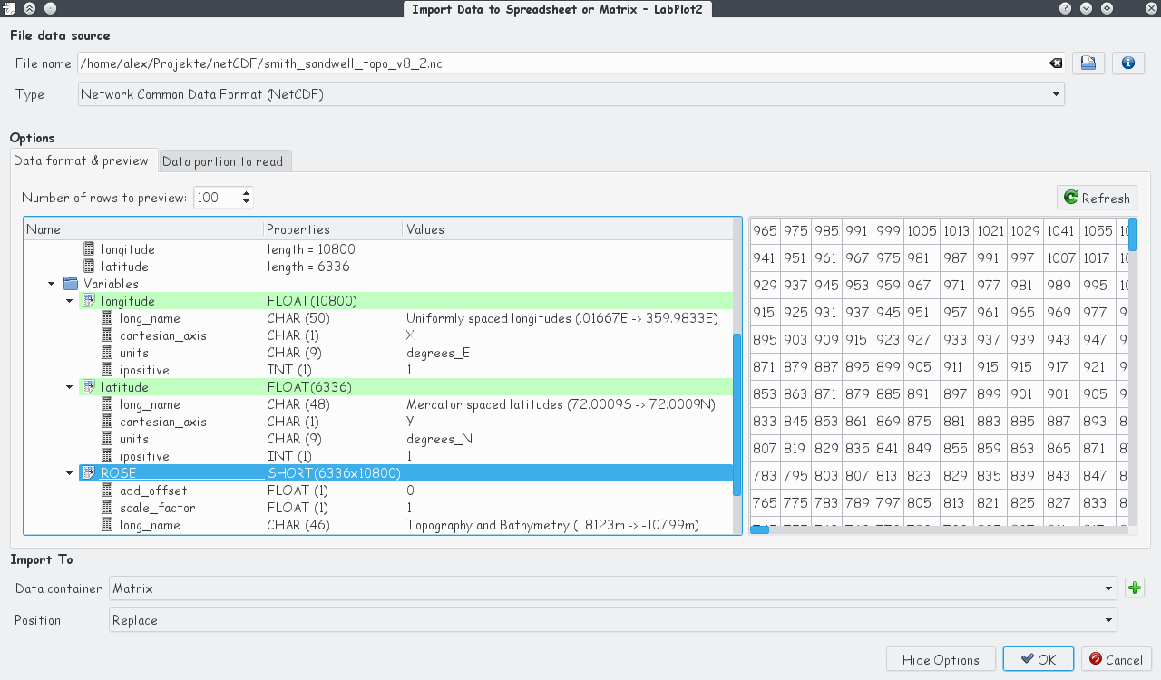
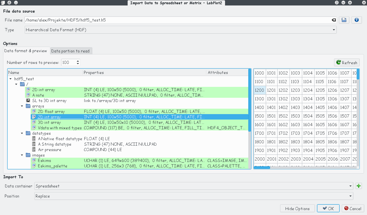
Import of external data into LabPlot was greatly extended. New data formats – binary, image, NetCDF and HDF5 – are supported now. Preview of all supported file types in the import dialog was improved. For data formats with complex internal structures like NetCDF and HDF5, the content of the file is presented in a tree view that allows comfortable navigation through the file. The screenshots below show two examples for a NetCDF-file (136.9MB) and for a HDF5-file (1.6MB):
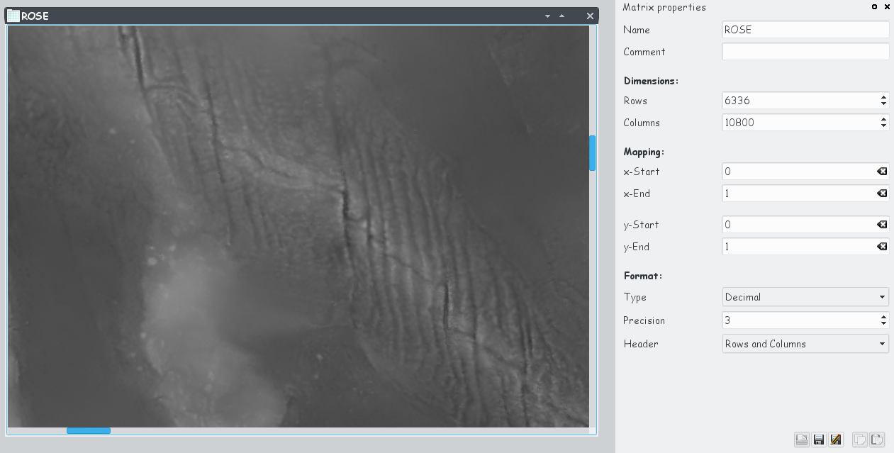
The next screenshot shows the data set ROSE from the example NetCDF-file mentioned above that was imported in LabPlot into a matrix, the image view was used.
The next new feature related to the data import improves the handling of compressed files. Import of data compressed with gzip, bzip2 or xz can be done now directly – the decompression happens transparently for the user.
2D-Plotting:
We’re still in the process of completing the 2D-plotting part of the application. Though this part is already very feature-rich in LabPlot, there’re still couple of gaps and we close some of them in this release.
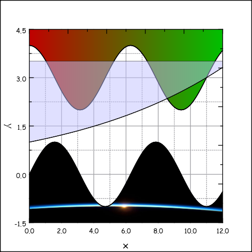
We implemented curve filling – the area below, under, left to or right to the curve can be filled with a solid color, a color gradient or with a user specified image.
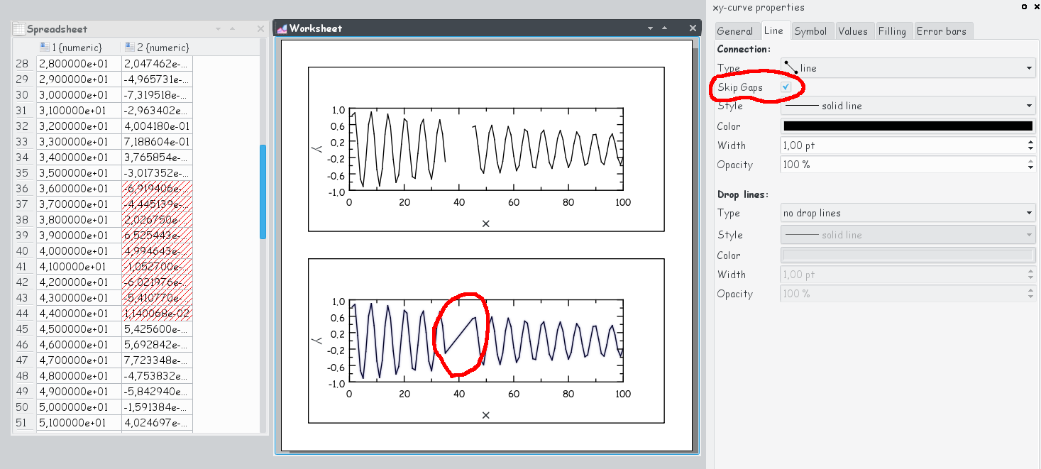
Sometimes there’re gaps in the data set – no values are available or some values don’t have a valid numerical format (“not a number”). When plotting such a data set it is often desirable not to interpolate between the data points in the region with missing data. This is now the default behavior in LabPlot that can be changes via the option “Skip Gaps”. The screenshot below shows two data sets with some masked data that was plotted with the option “Skip Gaps” switched off and on, respectively.
For the format of axis ticks, multiples of Pi can be used now – useful when plotting periodical functions. Minh Ngo, one of the three GSoC-students who worked this summer on LabPlot, contributed this small feature when he started to become familiar with LabPlot’s code.